How To Weight Variables In Machine Learning Python

Parametric vs Non-Parametric Learning Algorithms

Parametric — In a Parametric Algorithm, we have a fixed set of parameters such as theta that we effort to find(the optimal value) while training the data. After nosotros have establish the optimal values for these parameters, we can put the data aside or erase information technology from the computer and just use the model with parameters to make predictions. Call back, the model is only a function.

Non-Parametric — In a Non-Parametric Algorithm, you e'er accept to keep the data and the parameters in your estimator memory to make predictions. And that'southward why this type of algorithm may not exist great if you have a really really massive dataset.

Locally Weighted Linear Regression

Let the states apply the post-obit randomly generated data every bit a motivational case to empathize the Locally weighted linear regression.

                      import numpy as np                                np.random.seed(8)                                10 = np.random.randn(1000,1)
y = two*(Ten**three) + ten + 4.half-dozen*np.random.randn(1000,1)

In Linear Regression we would fit a straight line to this data but that won't piece of work here because the information is non-linear and our predictions would end up having large errors. We need to fit a curved line then that our fault is minimized.

Notations —

due north → number of features (1 in our instance)

one thousand → number of training examples (1000 in our example)

X(Uppercase) → Features

y → output sequence

x (lowercase)→ The point at which we want to make the prediction. Referred every bit point in the code.

x(i) →ith training example

In Locally weighted linear regression, we give the model the 10 where we desire to make the prediction, then the model gives all the x(i)'s around that x a higher weight close to ane, and the rest of x(i)'south get a lower weight shut to naught and so tries to fit a straight line to that weighted x(i)'s data.

This ways that if want to make a prediction for the dark-green indicate on the x-axis (see Effigy-one below), the model gives higher weight to the input data i.e. x(i)'south near or around the circumvolve above the green point and all else x(i) get a weight close to zero, which results in the model fitting a directly line only to the data which is nigh or close to the circle. The aforementioned goes for the imperial, xanthous, and grey points on the x-axis.

Ii questions come to listen afterwards reading that —

How to assign the weights?
How big should the circle be?

Weighting function (due west(i) →weight for the ith grooming example)

In Linear regression, nosotros had the following loss function —

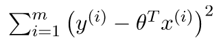
Loss Part for Linear Regression; source: geeksforgeeks.org

The modified loss for locally weighted regression —

Loss Function for Locally weighted Linear Regression; source: geeksforgeeks.org

w(i) (the weight for the ith training example) is the only modification.

where,

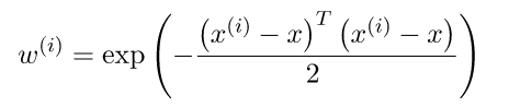
The weighting Function; source: geeksforgeeks.org

x is the signal where we want to make the prediction. x(i) is the ith training case.

The value of this role is always between 0 and 1.

And then, if we await at the role, we see that

If |10(i)-10| is pocket-size, w(i) is close to 1.
If |x(i)-x| is big, w(i) is shut to 0.

The x(i)'s which are far from x go w(i) close to nix and the ones which are shut to 10, go w(i) close to 1.

In the loss function, it translates to error terms for the x(i)'due south which are far from x being multiplied past virtually zero and for the x(i)'southward which are close to x get multiplied past almost i. In short, it only sums over the error terms for the x(i)'s which are close to x.

How big should the circumvolve be?

We introduce a hyperparameter tau in the weighting office which decided how large the circle should be.

Weighting Role with `tau;` source: geeksforgeeks.org

By changing the value of tau we can choose a fatter or a thinner width for circles.

For the math people here, tau is the bandwidth of the Gaussian bell-shaped bend of the weighing part.

Allow's code the weighting matrix. Run across comments (#).

          # Weight Matrix in lawmaking. It is a diagonal matrix.                      def wm(point, X, tau):                            # tau --> bandwidth
              # X --> Training data.
              # point --> the x where we want to make the prediction.
                            # one thousand is the No of training examples .
                              grand = X.shape[0]                          
                            # Initialising W as an identity matrix.
              w = np.mat(np.eye(chiliad))                          
                            # Calculating weights for all training examples [x(i)'s].
              for i in range(m):                
                11 = X[i]                
                d = (-2 * tau * tau)                
                w[i, i] = np.exp(np.dot((eleven-indicate), (11-point).T)/d)                
                      return w

Finally, The Algorithm

Actually, there exists a closed-form solution for this algorithm which means that we practise not accept to train the model, we tin can directly calculate the parameter theta using the post-obit formula.

Airtight-course solution for theta; source: geeksforgeeks.org

How to summate theta Do you ask?

Just take the fractional derivative of the modified loss function with respect to theta and gear up it equal to zero. And then, do a little fleck of linear algebra to become the value of theta.

For reference — Airtight-form solution for locally weighted linear regression

And after calculating theta, we can just apply the following formula to predict.

The formula for prediction; source: geeksforgeeks.org

Let'south code a predict role. Come across comments (#)

                      def predict(X, y, betoken, tau):                                         # m = number of preparation examples.              
                              thousand = X.shape[0]                          
                             # Appending a cloumn of ones in X to add the bias term.
## # But 1 parameter: theta, that's why calculation a column of ones        #### to X and also calculation a 1 for the point where we want to          #### predict.              
                              X_ = np.append(X, np.ones(thousand).reshape(yard,1), axis=ane)                
                            
              # point is the 10 where we want to make the prediction.              
                              point_ = np.assortment([point, 1])                
                            
              # Calculating the weight matrix using the wm function we wrote      #  # before.              
                              w = wm(point_, X_, tau)                
                            
              # Calculating parameter theta using the formula.
                              theta = np.linalg.pinv(X_.T*(due west * X_))*(X_.T*(w * y))                
                            
              # Computing predictions.              
                              pred = np.dot(point_, theta)                
                            
              # Returning the theta and predictions              
                              return theta, pred

Plotting Predictions

At present, allow's plot our predictions for most 100 points(x) which are in the domain of x.

See comments (#)

                      def plot_predictions(X, y, tau, nval):                                # X --> Training data.            
            # y --> Output sequence.
            # nval --> number of values/points for which nosotros are going to
            # predict.                      # tau --> the bandwidth.            
            # The values for which we are going to predict.
            # X_test includes nval evenly spaced values in the domain of X.
                          X_test = np.linspace(-3, 3, nval)              
                        
            # Empty listing for storing predictions.            


                          preds = []              
                        
            # Predicting for all nval values and storing them in preds.            
            for indicate in X_test:              
              theta, pred = predict(Ten, y, point, tau)              
              preds.append(pred)                             # Reshaping X_test and preds
                              X_test = np.array(X_test).reshape(nval,i)
                preds = np.array(preds).reshape(nval,1)            
                             # Plotting              
                              plt.plot(Ten, y, 'b.')
                plt.plot(X_test, preds, 'r.')              # Predictions in red color.                
                plt.show()            
                                plot_predictions(Ten, y, 0.08, 100)